
7.4 Multiple Layer Analysis
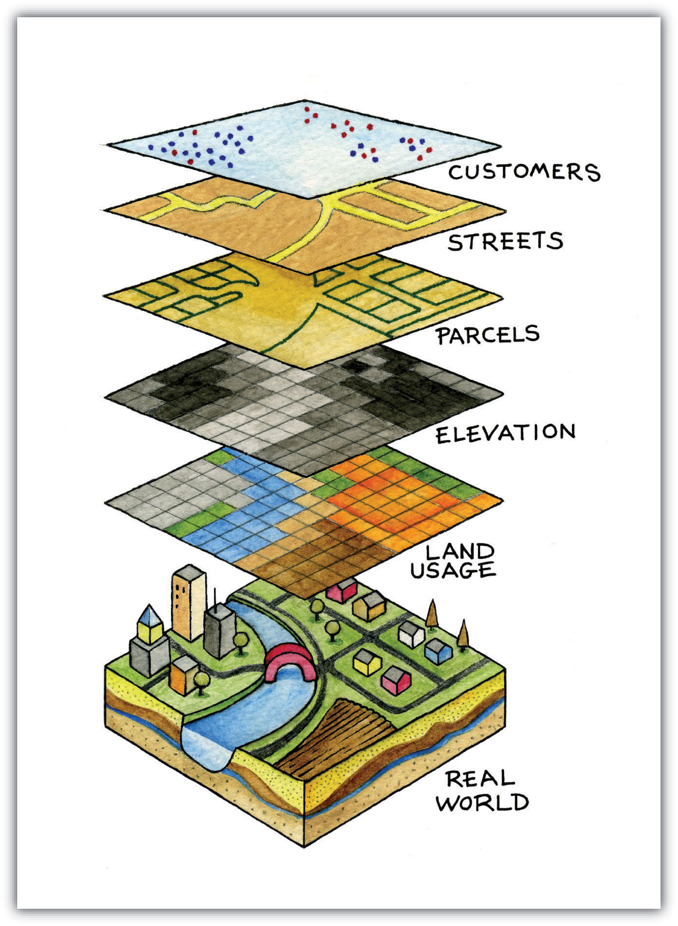
The overlay of cartographic information is among the most powerful and commonly used tools in a geographic information system (GIS). In a GIS, an overlay is a process of taking two or more different thematic maps of the same area and placing them on top of one another to form a new map. Inherent to this process, the overlay function combines the spatial features of the dataset and the attribute information.
A typical example of the overlay process is, “Where is the best place to put a mall?” Imagine you are a corporate bigwig tasked with determining where your company’s next shopping mall will be. How would you attack this problem? With a GIS at your command, answering such spatial questions begins with amassing and overlaying pertinent spatial data layers. For example, you may first want to determine what areas can support the mall by accumulating information on land parcels for sale and zoned for commercial development.
After collecting and overlaying the baseline information on available development zones, you can determine which areas offer the most economic opportunity by collecting regional information on average household income, population density, location of proximal shopping centers, local buying habits, and more. Next, you may want to collect information on restrictions or roadblocks to development, such as the cost of land, cost to develop the land, community response to the development, adequacy of transportation corridors to and from the proposed mall, tax rates, and so forth. Indeed, simply collecting and overlaying spatial datasets provides a valuable tool for visualizing and selecting the optimal site for such a business endeavor.
Overlay Operations
Several basic overlay processes are available in a GIS for vector datasets: point-in-polygon, polygon-on-point, line-on-line, line-in-polygon, polygon-on-line, and polygon-on-polygon. As you may be able to divine from the names, one of the overlay datasets must always be a line or polygon layer, while the second may be a point, line, or polygon. The new layer produced following the overlay operation is termed the “output” layer.
Point-in-Polygon Overlay Operation
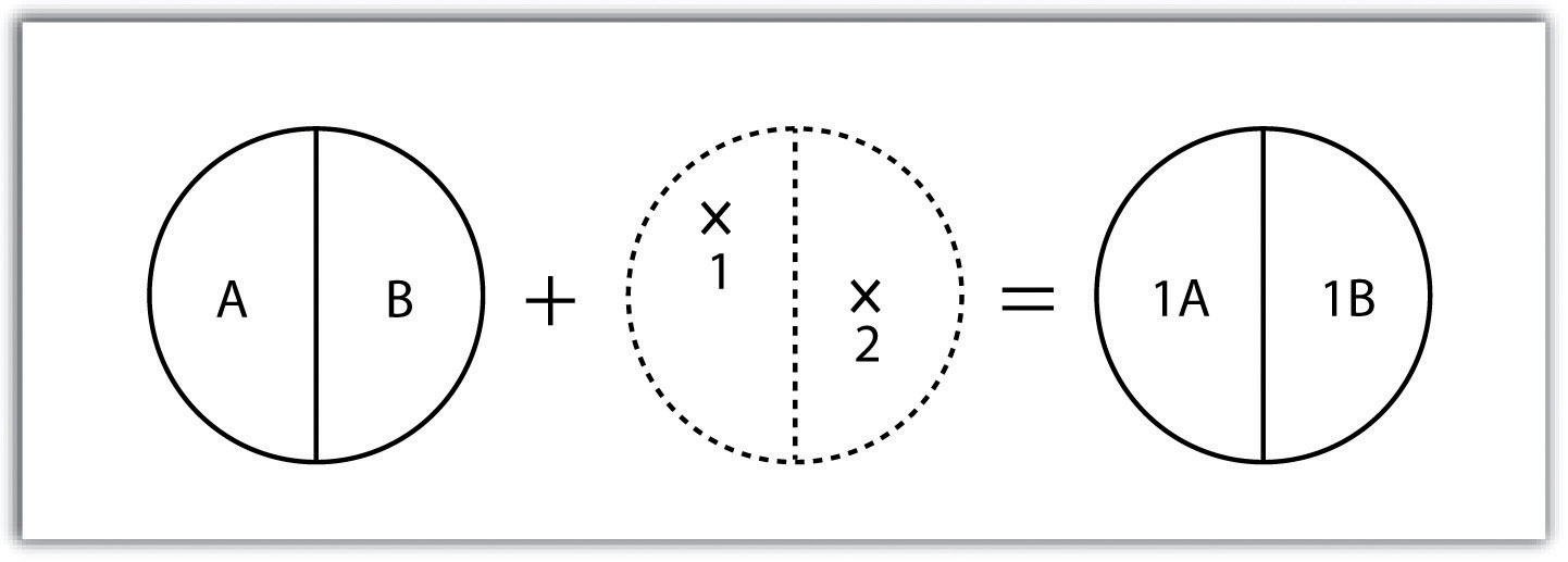
The point-on-polygon overlay operation requires a point input layer and a polygon layer. Upon performing this operation, a new output point layer is returned that includes all the points within the spatial extent of the overlay. In addition, all the points in the output layer contain their original attribute information and the attribute information from the overlay. For example, suppose you were tasked with determining if an endangered species residing in a national park was found primarily in a particular vegetation community. The first step would be to acquire the point occurrence locales for the species in question, plus a polygon overlay layer showing the vegetation communities within the national park boundary. Upon performing the point-in-polygon overlay operation, a new point file contains all the points within the national park. The attribute table of this output point file would also contain information about the vegetation communities being utilized by the species at the time of observation. A quick scan of this output layer and its attribute table would allow you to determine where the species was found in the park and review the vegetation communities in which it occurred. This process would enable park employees to make informed management decisions regarding which onsite habitats to protect to ensure continued site utilization by the species.
Polygon-on-Point Overlay Operation
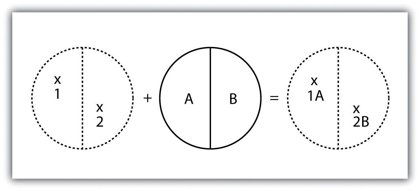
The polygon-on-point overlay operation is the opposite of the point-in-polygon operation. In this case, the polygon layer is the input, while the point layer is the overlay. The polygon features overlay these points selected and preserved in the output layer. For example, given a point dataset containing the locales of some crime and a polygon dataset representing city blocks, a polygon-on-point overlay operation would allow police to select the city blocks in which crimes have been known to occur and hence determine those locations where an increased police presence may be warranted.
Line-on-Line Overlay Operation
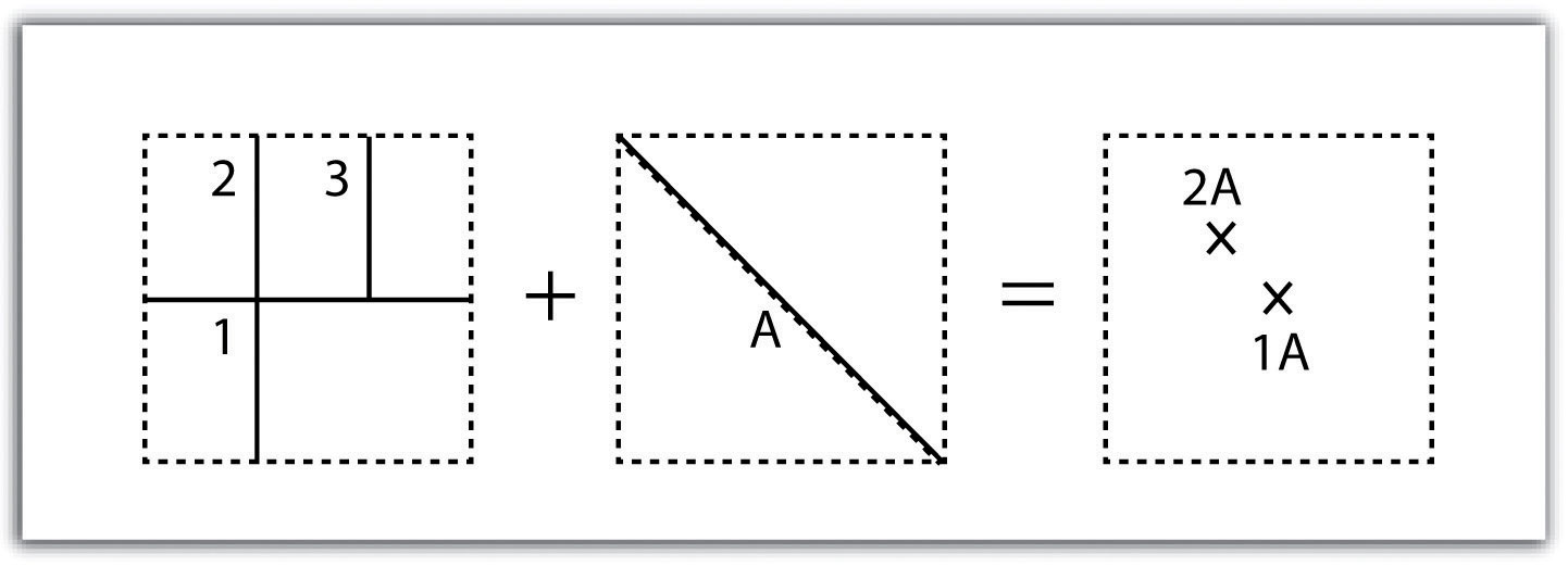
A line-on-line overlay operation requires line features for the input and overlay layer. The output from this operation is a point or points located precisely at the intersection(s) of the two linear datasets. For example, a linear feature dataset containing railroad tracks may be overlaid on a linear road network. The resulting point dataset contains all the locales of the railroad crossings over a town’s road network. The attribute table for this railroad crossing point dataset would contain information on the railroad and the road it passed.
The line-in-polygon overlay operation is similar to the point-in-polygon overlay, with the obvious exception that a line input layer is used instead of a point input layer. In this case, each line that has any part of its extent within the overlay polygon layer will be included in the output line layer, although these lines will be truncated at the boundary of the overlay. For example, a line-in-polygon overlay can take an input layer of interstate line segments and a polygon overlay representing city boundaries and produce a linear output layer of highway segments within the city boundary. The attribute table for the output interstate line segment will contain information on the interstate name and the city through which they pass.
Polygon-on-Line Overlay Operation
The polygon-on-line overlay operation is the opposite of the line-in-polygon operation. In this case, the polygon layer is the input, while the line layer is the overlay. The polygon features overlay these lines are selected and subsequently preserved in the output layer. For example, given a layer containing the path of a series of telephone poles/wires and a polygon map containing city parcels, a polygon-on-line overlay operation would allow a land assessor to select those parcels containing overhead telephone wires.
Polygon-in-Polygon Overlay Operation
Finally, the polygon-in-polygon overlay operation employs a polygon input and a polygon overlay. This is the most commonly used overlay operation. This method combines the polygon input and overlay layers to create an output polygon layer with the extent of the overlay. The attribute table will contain spatial data and attribute information from the input and overlay layers. For example, you may choose an input polygon layer of soil types with an overlay of agricultural fields within a given county. The output polygon layer would contain information on the location of agricultural fields and soil types throughout the county.
The overlay operations discussed previously assume that the user desires to combine the overlain layers. This is not always the case. Overlay methods can be more complex and employ the basic Boolean operators: AND, OR, and XOR. Depending on which operator(s) are utilized, the overlay method will result in an intersection, union, symmetrical difference, or identity.
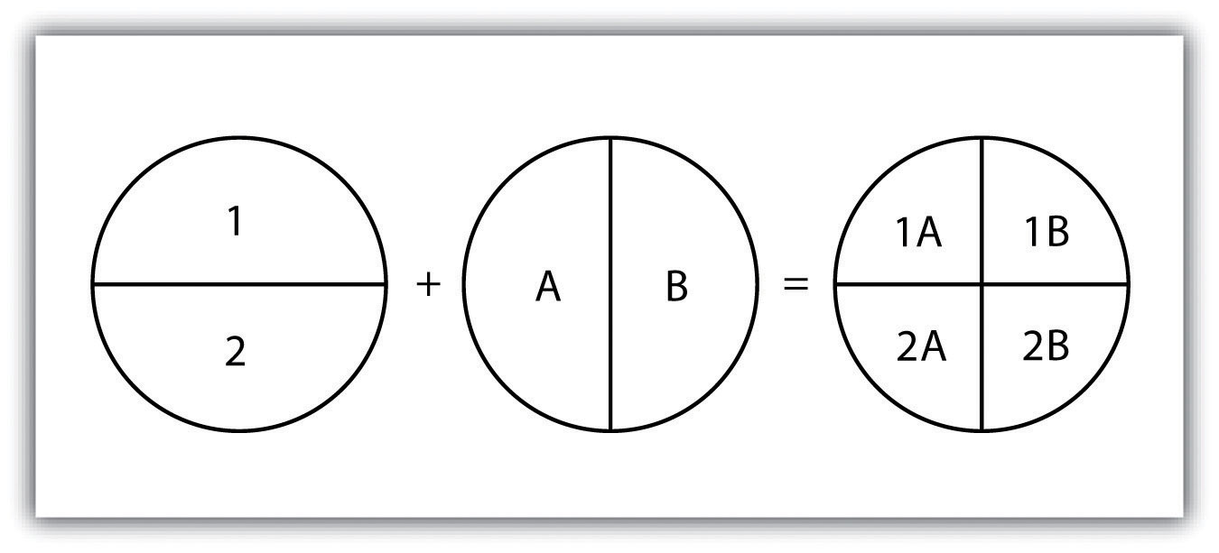
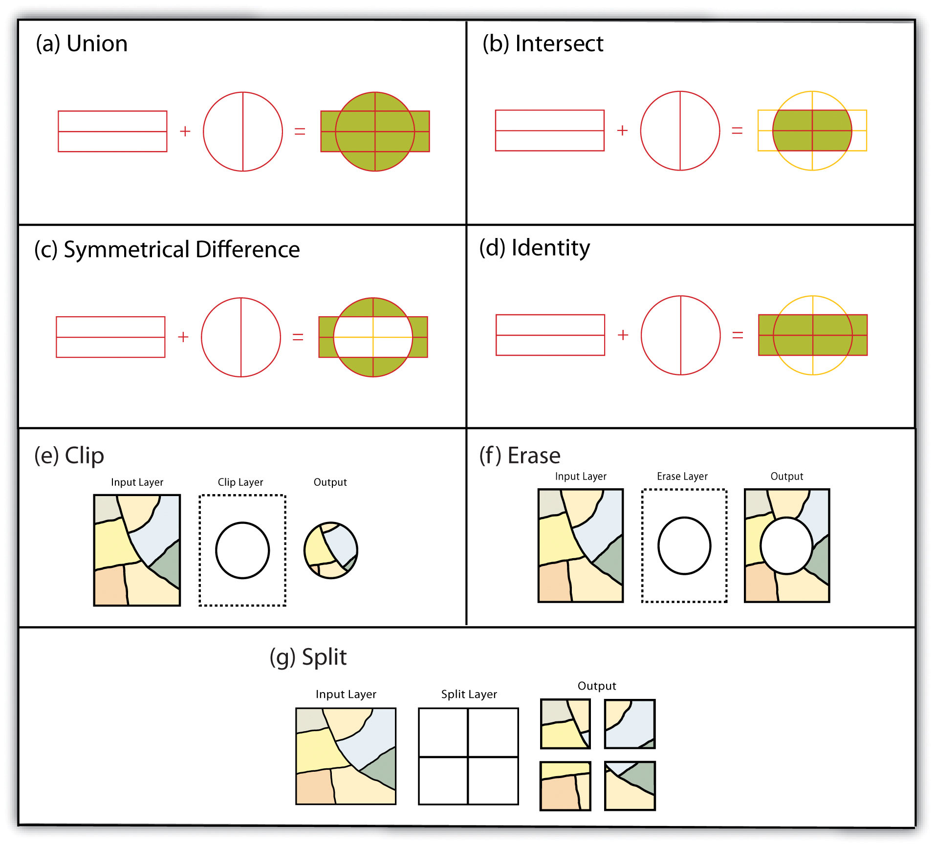
Specifically, the union overlay method employs the OR operator. A union can be used only in the case of two polygon input layers. It preserves all features, attribute information, and spatial extents from both input layers. This overlay method is based on the polygon-in-polygon operation.
Alternatively, the intersection overlay method employs the AND operator. An intersection requires a polygon overlay but can accept a point, line, or polygon input. The output layer covers the spatial extent of the overlay and contains features and attributes from both the input and overlay.
The symmetrical difference overlay method employs the XOR operator, which results in the opposite output as an intersection. This method requires both input layers to be polygons. The output polygon layer produced by the symmetrical difference method represents those areas common to only one of the feature datasets.
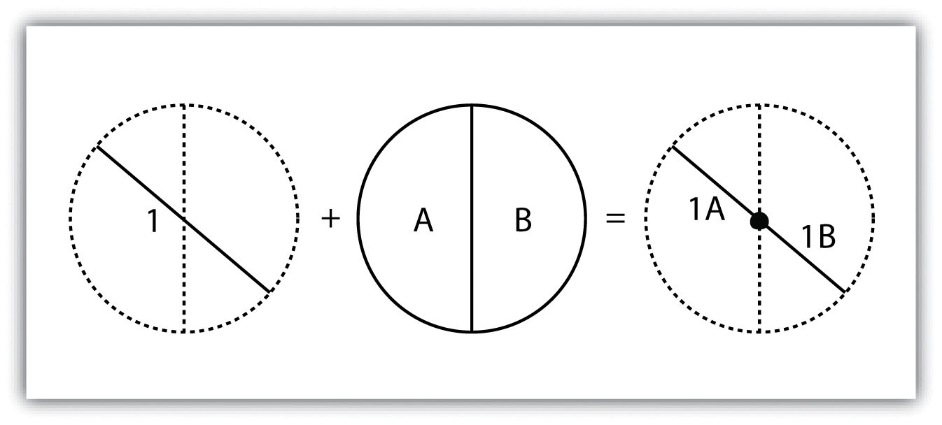
In addition to these simple operations, the identity overlay method creates an output layer with the spatial extent of the input layer but includes attribute information from the overlay (referred to as the “identity” layer, in this case). The input layer can be points, lines, or polygons. The identity layer must be a polygon dataset.
Other Multilayer Geoprocessing Options
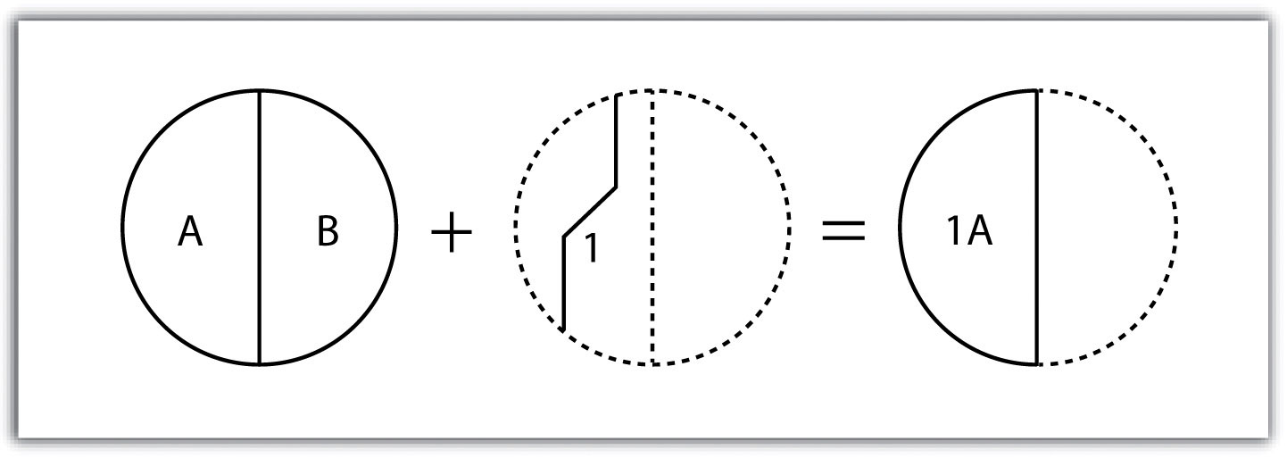
In addition to the vector mentioned above overlay methods, other standard multiple-layer geoprocessing options are available to the user. These included the clip, erase, and split tools. The clip geoprocessing operation extracts those features from an input point, line, or polygon layer that falls within the spatial extent of the clip layer. Following the clip, all attributes from the preserved portion of the input layer are included in the output. If any features are selected during this process, only those selected features within the clip boundary will be included in the output. For example, the clip tool could clip the extent of a river floodplain by the extent of a county boundary. This would give county managers insight into which portions of the floodplain they are responsible for maintaining. This is similar to the intersect overlay method; however, the attribute information associated with the clip layer is not carried into the output layer following the overlay.
The erase geoprocessing operation is essentially the opposite of a clip. Whereas the clip tool preserves areas within an input layer, the erase tool preserves only those areas outside the extent of the analogous erase layer. While the input layer can be a point, line, or polygon dataset, the erase layer must be a polygon dataset. Continuing with our clip example, county managers could then use the erase tool to erase the areas of private ownership within the county floodplain area. Officials could then focus specifically on the public reaches of the countywide floodplain for their upkeep and maintenance responsibilities.
The split geoprocessing operation divides an input layer into two or more layers based on a split layer. The split layer must be a polygon, while the input layers can be a point, line, or polygon. For example, a homeowner’s association may choose to split up a countywide soil series map by parcel boundaries, so each homeowner has a specific soil map for their parcel.
Spatial Join
A spatial join is a hybrid between an attribute operation and a vector overlay operation. Like the “join” attribute operation, a spatial join combines two feature dataset tables by a common attribute field. However, unlike the attribute operation, a spatial join determines which fields from a source layer’s attribute table are appended to the destination layer’s attribute table based on the relative locations of selected features. This relationship is explicitly based on the property of proximity or containment between the source and destination layers rather than the primary or secondary keys. The proximity option is used when the source layer is a point or line feature dataset, while the containment option is used when the source layer is a polygon feature dataset.
When employing the proximity (or “nearest”) option, a record for each feature in the source layer’s attribute table is appended to the closest given feature in the destination layer’s attribute table. In addition, the proximity option will typically add a numerical field to the destination layer attribute table, called “Distance,” within which the measured distance between the source and destination feature is placed. For example, suppose a city agency had a point dataset showing all known polluters in town and a line dataset of all the river segments within the municipal boundary. This agency could then perform a proximity-based spatial join to determine the nearest river segment that each polluter would likely affect.
When using the containment (or “inside”) option, a record for each feature in the polygon source layer’s attribute table is appended to the record in the destination layer’s attribute table. No value will be appended if a destination layer feature (point, line, or polygon) is not entirely contained within a source polygon. For example, suppose a pool cleaning business wanted to hone its marketing services by providing flyers only to homes that owned a pool. First, they could obtain a point dataset containing every county pool’s location and a polygon parcel map for that area. Then, that business could conduct a spatial join to ap-pend the parcel information to the pool locales. This would provide them with information on each land parcel that contained a pool, and they could subsequently send their mailers only to those homes.
Overlay Errors
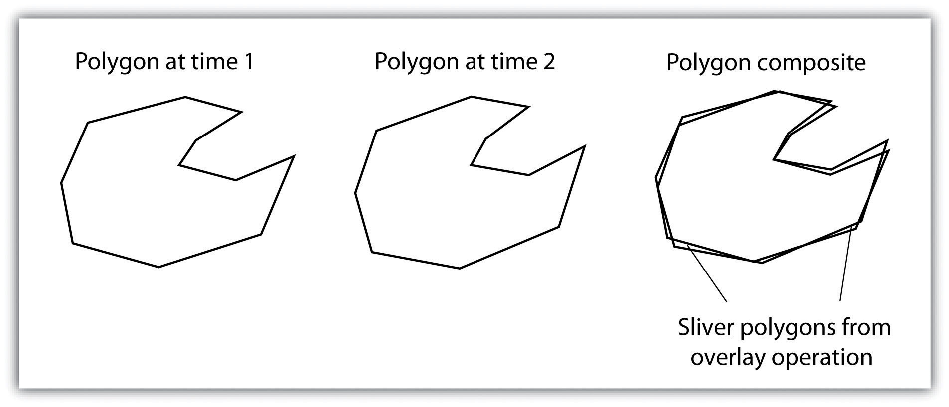
Although overlays are one of the essential tools in a GIS analyst’s toolbox, some problems can arise when using this methodology. In particular, slivers are a standard error produced when two slightly misaligned vector layers overlap. This misalignment can come from several sources, including digitization, interpretation, or source map errors (Chang, 2008). For example, most vegetation and soil maps are created from field survey data, satellite images, and aerial photography. While you can imagine that the boundaries of soils and vegetation frequently coincide, the fact that different researchers most likely created them at different times suggests that their boundaries will not overlap perfectly. GIS software incorporates a cluster tolerance option that forces nearby lines to be snapped together if they fall within a user-specified distance to ameliorate this problem. Care must be taken when assigning cluster tolerance. Too strict a setting will not snap shared boundaries, while too lenient a setting will snap unintended, neighboring boundaries together (Wang & Donaghy, 1995).
Error propagation is a second potential source of error associated with the overlay process. Error propagation arises when inaccuracies are present in the original input and overlay layers and are propagated through to the output layer (MacDougall, 1975). For example, these errors can be related to positional inaccuracies of the points, lines, or polygons. In addition, they can arise from attribute errors in the original data table(s). Regardless of the source, error propagation represents a common problem in overlay analysis, which depends mainly on the accuracy and precision requirements of the project at hand.
Click the “Previous” button on the lower left or the ‘Next” button on the lower right to navigate throughout the textbook.
