Single-layer analyses are undertaken on an individual GIS feature dataset. Buffering is creating an output polygon layer containing a zone (or zones) of a specified width around an input point, line, or polygon feature. Buffers are particularly suited for determining the influence area around interest features. Geoprocessing is a suite of tools provided by geographic information system (GIS) software packages that allow users to automate many mundane tasks associated with manipulating GIS data. Geoprocessing usually involves the input of one or more feature datasets, followed by a spatially explicit analysis, resulting in an output feature dataset.

Buffering

Buffers are standard vector analysis tools used to address questions of proximity in a GIS and can be used on points, lines, or polygons. For instance, suppose that a natural resource manager wants to ensure that no areas are disturbed within 1,000 feet of the breeding habitat for the federally endangered Delhi Sands flower-loving fly. Unfortunately, this species is found only in the few remaining Delhi Sands soil formations of the western United States. To accomplish this task, a 1,000-foot protection zone (buffer) could be created around all the observed point locations of the species. Alternatively, the manager may decide that there is insufficient point-specific location information related to this rare species and decide to protect all of Delhi Sands’ soil formations. In this case, he or she could create a 1,000-foot buffer around all polygons labeled “Delhi Sands” on a soil formations dataset. In either case, buffers provide a quick-and-easy tool for determining which areas are to be maintained as preserved habitats for the endangered fly.

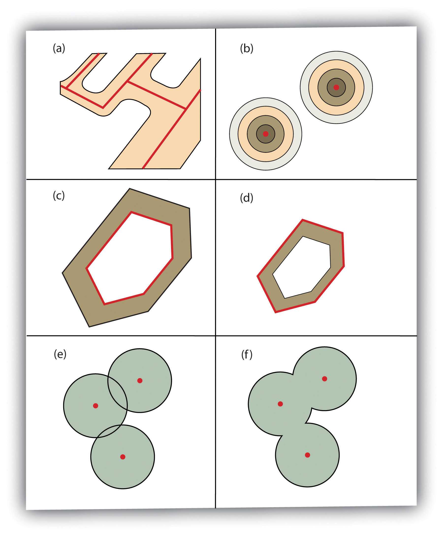
Several buffering options are available to refine the output. For example, the buffer tool will typically buffer only selected features. If no features are selected, all features will be buffered. Two primary buffers are available to GIS users: constant width and variable width. Constant width buffers require users to input a value by which features are buffered (Figure 7.1 “Buffers around Red Point, Line, and Polygon Features”), as seen in the preceding paragraph examples. Variable width buffers, on the other hand, call on a premade buffer field within the attribute table to determine the buffer width for each specific feature in the dataset (Figure 7.2 “Additional Buffer Options around Red Features: (a) Variable Width Buffers, (b) Multiple Ring Buffers, (c) Doughnut Buffer, (d) Setback Buffer, (e) Nondissolved Buffer, (f) Dissolved Buffer”).

In addition, users can choose to dissolve or not dissolve the boundaries between overlapping, coincident buffer areas. For example, multiple ring buffers can be made such that a series of concentric buffer zones (much like an archery target) is created around the originating feature at user-specified distances. In the case of polygon layers, buffers can be created that includes the originating polygon feature as part of the buffer, or they are created as a doughnut buffer that excludes the input polygon area. Setback buffers are similar to doughnut buffers; however, they only buffer the area inside the polygon boundary. For example, linear features can be buffered on both sides of the line, only on the left or right. Line-ar features can also be buffered so that the endpoints of the line are rounded (ending in a half-circle) or flat (ending in a rectangle).

Geoprocessing Operations

The term geoprocessing is widely applied to any attempt to manipulate GIS data. However, the term came into common usage due to its application to a somewhat arbitrary suite of single-layer and multiple-layer analytical techniques in the Geoprocessing Wizard of ESRI’s ArcView software package in the mid-1990s. Regardless, the suite of geoprocessing tools available in a GIS greatly expands and simplifies many of the management and manipulation processes associated with vector feature datasets. These tools primarily automate the repetitive preprocessing needs of typical spatial analyses and assemble exact graphical representations for subsequent analysis and inclusion in presentations and final mapping products. These geoprocessing tools often use the union, intersect, symmetrical difference, and identity overlay methods. The following represents the most common geoprocessing tools.

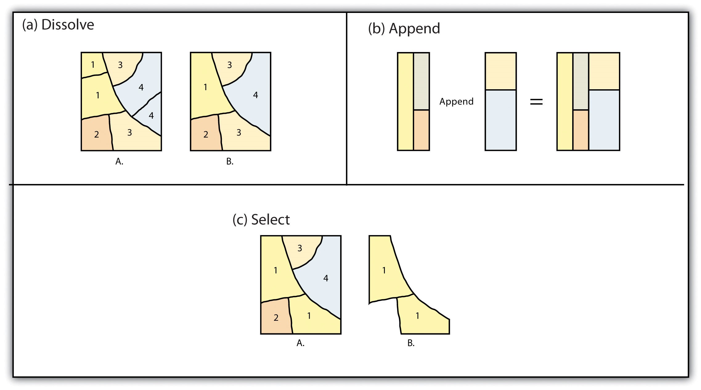
The dissolve operation combines adjacent polygon features in a single feature dataset based on a predetermined attribute. For example, part (a) of figure 7.3, “Single Layer Geo-processing Functions,” shows the boundaries of seven different parcels of land owned by four different families (labeled 1 through 4). The dissolve tool automatically combines all adjacent features with the same attribute values. The result is an output layer with the same extent as the original but without all of the unnecessary, intervening line segments. The dis-solved output layer is easier to visually interpret when the map is classified according to the dissolved field.

The append operation creates an output polygon layer by combining the spatial extent of two or more layers (part (d) of Figure 7.3 “Single Layer Geoprocessing Functions”). For use with point, line, and polygon datasets, the output layer will be the same feature type as the input layers (which must be the same feature type as well). Unlike the dissolve tool, the append does not remove the boundary lines between appended layers (in the case of lines and polygons). Therefore, performing a dissolve after using the append tool is often helpful in removing these potentially unnecessary dividing lines. Append is frequently used to mosaic data layers, such as digital US Geological Survey (USGS) 7.5-minute topographic maps, to create a single map for analysis and display.

The select operation creates an output layer based on a user-defined query that selects particular features from the input layer (part (f) of Figure 7.3 “Single Layer Geoprocessing Functions”). The output layer contains only those features that are selected during the query. For example, a city planner may select all zoned “residential” areas to quickly assess which areas in town are suitable for proposed housing development.

Finally, the merge operation combines features within a point, line, or polygon layer into a single feature with identical attribute information. Often, the original features will have different values for a given attribute. The first attribute encountered is carried over into the attribute table, and the remaining attributes are lost. This operation is beneficial when polygons are found to be unintentionally overlapping. Merge will conveniently combine these features into a single entity.

Click the “Previous” button on the lower left or the ‘Next” button on the lower right to navigate throughout the textbook.