In contrast, the raster data model is the vector data model. This model does not quantify space into discrete grid cells like the raster model. Instead, vector data models use points and their associated X and Y coordinate pairs to represent the vertices of spatial features as if they were being drawn on a map by hand (Aronoff, 1989). Aronoff, S. 1989. Geographic Information Systems: A Management Perspective. Ottawa, Canada: WDL Publications. The data attributes of these features are then stored in a separate database management system. Finally, these models’ spatial and attribute information are linked via a simple identification number given to each feature in a map.

Three fundamental vector types exist in geographic information systems (GISs): points, lines, and polygons. Points are zero-dimensional objects that contain only a single coordinate pair. Points are typically used to model singular, discrete features such as buildings, wells, power poles, and sample locations. Points have only the property of location. Other types of point features include the node and the vertex. Specifically, a point is a stand-alone feature, while a node is a topological junction representing a standard X and Y coordinate pair between intersecting lines or polygons. Vertices are defined as each bend along a line or polygon feature that is not the intersection of lines or polygons.

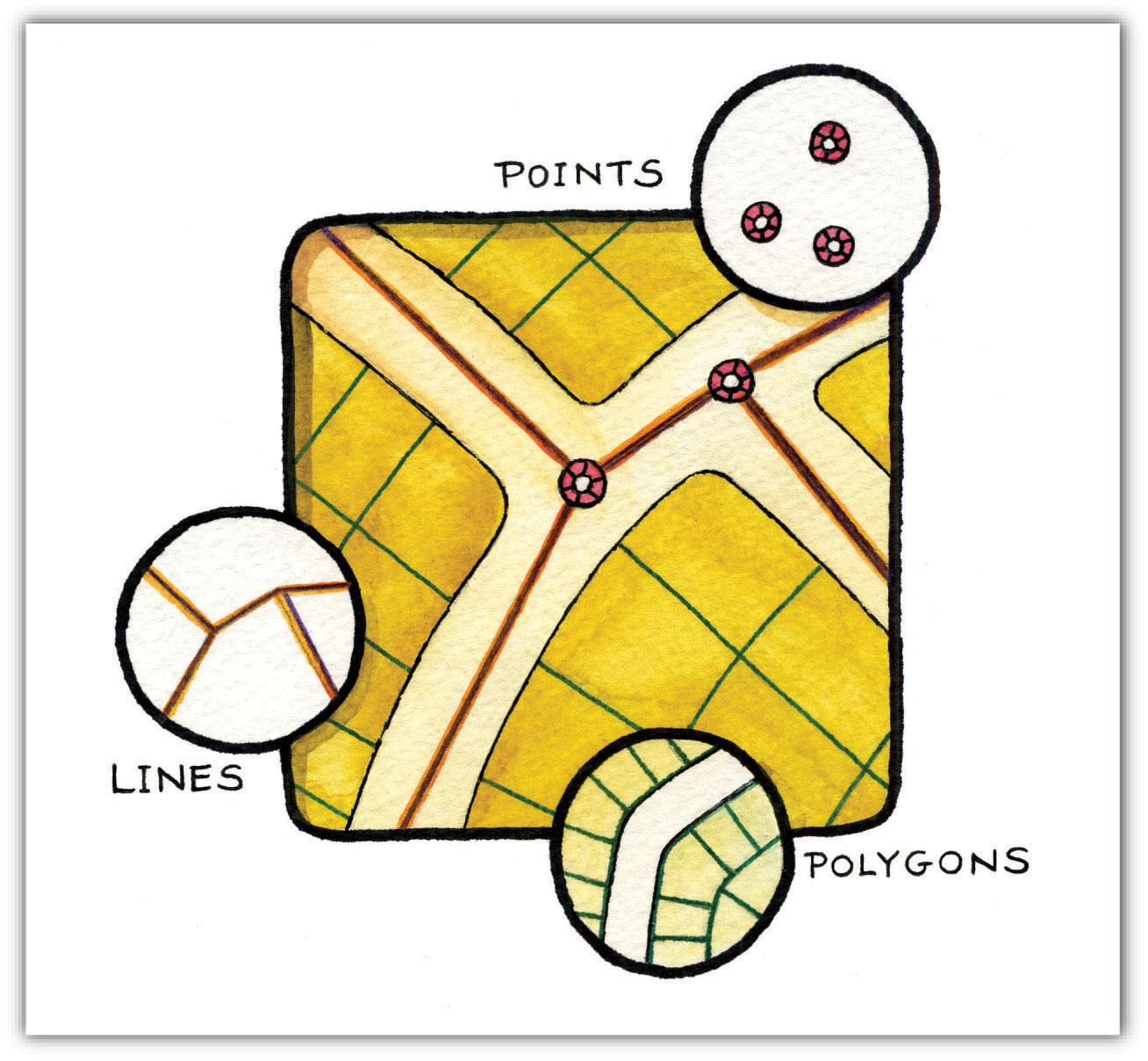
Points can be spatially linked to form more complex features. Lines are one-dimensional features composed of multiple, explicitly connected points. Lines represent linear features such as roads, streams, faults, and boundaries. Lines have the property of length. Lines connecting two nodes are sometimes called chains, edges, segments, or arcs.

Polygons are two-dimensional features created by multiple lines that loop back to create a “closed” feature. In the case of polygons, the first coordinate pair (point) on the first line segment is the same as the last coordinate pair on the last line segment. Polygons represent city boundaries, geologic formations, lakes, soil associations, vegetation communities, etc. In addition, polygons have the properties of area and perimeter. Therefore, polygons are also called areas.

Vector Data Model Structures

Vector data models can be structured in many different ways. We will examine two of the more common data structures here. The spaghetti data model is the simplest vector data structure (Dangermond, 1982). In the spaghetti model, each point, line, or polygon feature is represented as a string of X, Y coordinate pairs (or as a single X, Y coordinate pair in the case of a vector image with a single point) with no inherent structure (Figure 4.9 “Spaghetti Data Model”). One could envision each line in this model to be a single strand of spaghetti formed into complex shapes by adding more strands of spaghetti. In this model, any adjacent polygons must be made up of lines or spaghetti stands. In other words, each polygon must be uniquely defined by its own set of X and Y coordinate pairs, even if the adjacent polygons share the same boundary information. This creates some redundancies within the data model and therefore reduces efficiency.

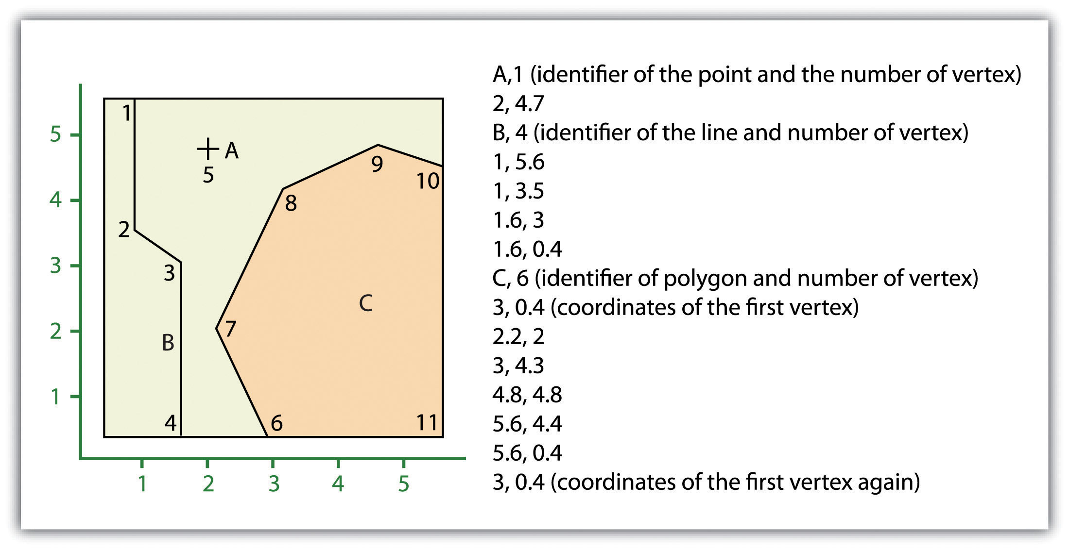
Despite the location designations associated with each line, or strand of spaghetti, spatial relationships are not explicitly encoded within the spaghetti model; instead, they are implied by their location. This results in a lack of topological information, which is problematic if the user attempts to make measurements or analyses. The computational requirements, therefore, are very steep if any advanced analytical techniques are employed on vector file structure. Nevertheless, the simple structure of the spaghetti data model allows for the efficient reproduction of maps and graphics, as this topological information is unnecessary for plotting and printing.

In contrast to the spaghetti data model, the topological data model is characterized by including topological information within the dataset, as the name implies. Topology is a set of rules that model the relationships between neighboring points, lines, and polygons and determines how they share geometry. For example, consider two adjacent polygons. In the spaghetti model, the shared boundary of two neighboring polygons is defined as two separate, identical lines. Including topology in the data, the model allows for a single line to represent this shared boundary with an explicit reference to denote which side of the line belongs with which polygon. Topology is also concerned with preserving spatial properties when the forms are bent, stretched, or placed under similar geometric transformations, which allows for more efficient projection and reprojection of map files.

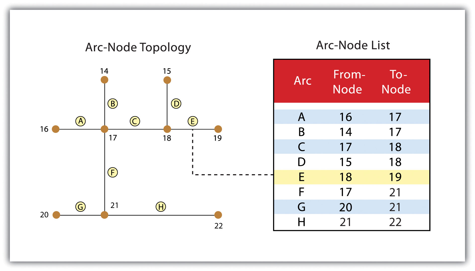
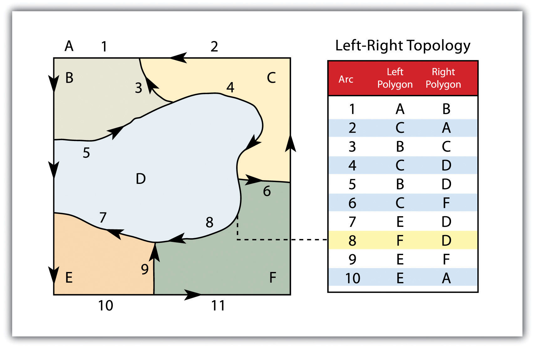
Three basic topological precepts are outlined here to understand the topological data model. First, connectivity describes the arc-node topology for the feature dataset. As discussed previously, nodes are more than simple points. In the topological data model, nodes are the intersection points where two or more arcs meet. In the case of arc-node topology, arcs have both a from-node (i.e., starting node) indicating where the arc begins and a to-node (i.e., ending node) indicating where the arc ends. In addition, between each node pair is a line segment, sometimes called a link, which has its identification number and references both its from-node and to-node. For example, in the figure below, arcs 1, 2, and 3 intersect because they share node 11. Therefore, the computer can determine that it is possible to move along arc 1 and turn onto arc 3, while it is impossible to move from arc 1 to arc 5, as they do not share a common node.

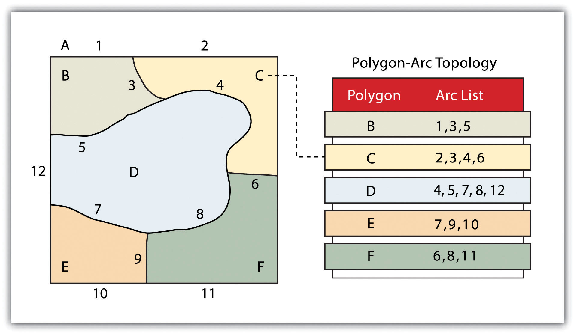
The second fundamental topological precept is area definition. Area definition states that an arc that connects to surround an area defines a polygon, also called polygon-arc topology. In the case of polygon-arc topology, arcs are used to construct polygons, and each arc is stored only once. This reduces the amount of data stored and ensures that adjacent polygon boundaries do not overlap. For example, the polygon-arc topology makes it clear that polygon F comprises arcs 8, 9, and 10.

Contiguity, the third topological precept, is based on the concept that polygons that share a boundary are deemed adjacent. Specifically, polygon topology requires that all arcs in a polygon have a direction (a from-node and a to-node), which allows adjacency information to be determined. Polygons that share an arc are deemed adjacent or contiguous; therefore, each arc’s “left” and “right” sides can be defined. This left and right polygon information is stored explicitly within the attribute information of the topological data model. The “universe polygon” is an essential component of polygon topology representing the external area outside the study area. The figure below shows that arc 6 is bound on the left by polygon B and to the right by polygon C. Polygon A, the universe polygon, is to the left of arcs 1, 2, and 3.

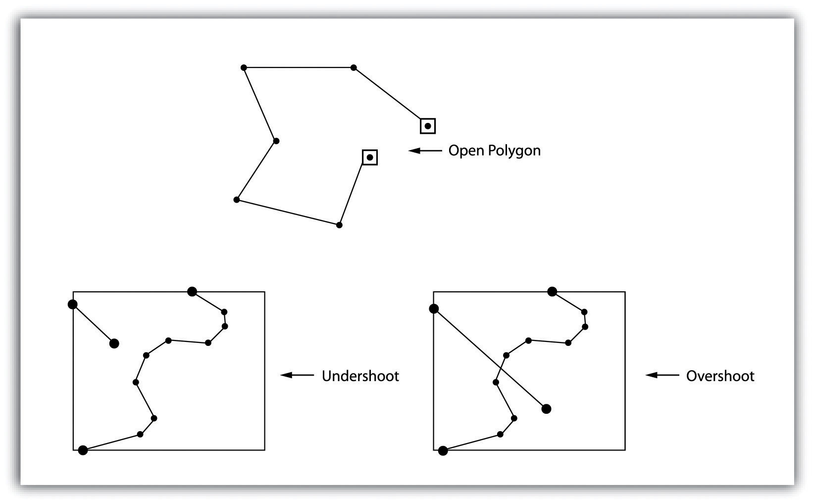
Topology allows the computer to rapidly determine and analyze the spatial relationships of all its included features. In addition, topological information is essential because it allows for efficient error detection within a vector dataset. In the case of polygon features, open or unclosed polygons, which occur when an arc does not completely loop back upon itself, and unlabeled polygons, which occur when an area does not contain any attribute information, violate polygon-arc topology rules. Another topological error found with polygon features is the sliver. Slivers occur when the shared boundary of two polygons does not meet precisely.

In the case of line features, topological errors occur when two lines do not meet perfectly at a node. This error is called an “undershoot” when the lines do not extend far enough to meet each other and an “overshoot” when the line extends beyond the feature it should connect to. The result of overshoots and undershoots is a “dangling node” at the end of the line. Dangling nodes are not always an error, however, as they occur in the case of dead-end streets on a road map.

Many types of spatial analysis require the degree of organization offered by topologically explicit data models. In particular, network analysis (e.g., finding the best route from one location to another) and measurement (e.g., finding the length of a river segment) relies heavily on the concept of to and from nodes. It uses this information and attributes information to calculate distances, shortest routes, quickest routes, and so forth. Topology also allows for sophisticated neighborhood analysis, such as determining adjacency, clustering, or nearest neighbors.

Now that the basics of the concepts of topology have been outlined, we can begin to understand the topological data model better. In this model, the node acts as more than just a simple point along a line or polygon. Instead, the node represents the point of intersection for two or more arcs. Arcs may or may not be looped into polygons. Regardless, all nodes, arcs, and polygons are individually numbered. This numbering allows for quick and easy reference within the data model.

Advantages and Disadvantages of Vector Models

In comparison with the raster data model, vector data models tend to be better representations of reality due to the accuracy and precision of points, lines, and polygons over the regularly spaced grid cells of the raster model. This results in vector data tending to be more aesthetically pleasing than raster data.

Vector data also provides an increased ability to alter the scale of observation and analysis. However, as each coordinate pair associated with a point, line, and polygon represents an infinitesimally exact location (albeit limited by the number of significant digits or data acquisition methodologies), zooming deep into a vector image does not change the view of a vector graphic in the way that it does a raster graphic.

Vector data tend to be more compact in the data structure, so file sizes are typically much smaller than their raster counterparts. Although the ability of modern computers has minimized the importance of maintaining small file sizes, vector data often require a fraction of the computer storage space compared to raster data.

The final advantage of vector data is that topology is inherent in the vector model. This topological information results in simplified spatial analysis (e.g., error detection, network analysis, proximity analysis, and spatial transformation) using a vector model.

Alternatively, there are two primary disadvantages of the vector data model. First, the data structure tends to be much more complex than the simple raster data model. As the location of each vertex must be stored explicitly in the model, there are no shortcuts for storing data like there are for raster models (e.g., the run-length and quad-tree encoding methodologies).

Second, the implementation of spatial analysis can also be relatively complicated due to minor differences in accuracy and precision between the input datasets. Similarly, the algorithms for manipulating and analyzing vector data are complex and can lead to intensive processing requirements, mainly when dealing with large datasets.

Click the “Previous” button on the lower left or the ‘Next” button on the lower right to navigate throughout the textbook.