Chapter 7: Basic Political Analysis

“The median black family, with just over $3,500, owns just 2 percent of the wealth of the nearly $147,000 the median white family owns. The median Latino family, with just over $6,500, owns just 4 percent of the wealth of the median white family. Put differently, the median white family has 41 times more wealth than the median black family and 22 times more wealth than the median Latino family.”

—Inequalty.org (1)

Calculating Percentages

Political scientists use basic and sophisticated quantitative and qualitative research methods in their work. Reviewing those methods is beyond the scope of this introductory text. Still, you should be familiar with the following basic analytical techniques.

One of the most basic operations we can do in quantitative analysis is to sort things into categories and count how many instances fit into each category. Another is to translate raw numbers into percentages. Let’s look at a subtle yet important change in the United States that is reflected in the number of associate’s and bachelor’s degrees conferred in the United States between 1970 and 2000. The National Center for Education Statistics has the following data for college degree attainment in those years. (2) Check out these facts:

• In 1970, colleges and universities conferred 206,000 associate’s degrees, of which 117,000 were to men and 89,000 were to women. In 2000, colleges and universities conferred 565,000 associate’s degrees, of which 225,000 were to men and 340,000 were to women.
• In 1970, colleges and universities conferred 792,000 bachelor’s degrees, of which 451,000 were to men and 341,000 were to women. In 2000, colleges and universities conferred 1,238,000 bachelor’s degrees, of which 530,000 were to men and 708,000 were to women.

Overall, we can see the growing popularity of higher education for both sexes in the United States. The number of associate’s degrees more than tripled during those three decades, while the number of bachelor’s degrees nearly doubled. But the really interesting story has to do with the proportion of degrees women and men received. Can you see it? If you look carefully you can. The difficulty in seeing what is happening is a common one with frequency distributions. Because the total number of degrees in each category changes year by year, it is not always easy to see patterns in the blizzard of raw numbers. What if we standardize the numbers by presenting degrees earned by men and women as percentages of the total number of degrees?

• In 1970, 57% of associate’s degrees were earned by men and 43% by women. By 2000, only 40% of associate’s degrees were earned by men and 60% by women.
• In 1970, 57% of bachelor’s degrees were earned by men and 43% by women. By 2000, only 43% of bachelor’s degrees were earned by men and 57% by women.

By converting the raw numbers to percentages, we gain better understanding of what happened in that period. We can clearly see that at both the associate’s and bachelor’s level, the percentage of degrees earned by women has grown since 1970 while the percentage earned by men has slipped. Even simple quantitative analysis such as this can be very powerful and can prompt political scientists and sociologists to dig deeper. What caused this shift? What political, social, and economic impacts did this shift produce? Can we find evidence of those impacts today?

It’s easier for the brain to figure out what’s happening here if we translate the raw numbers into percentages, because doing so highlights the actual proportion of degrees received by type per year. In this course, you absolutely, positively must be able to figure percentages.

The first thing to learn is calculating percentages that are less than 100%. An easy way to remind yourself how to do that is to remember the simple phrase, “part over total, times one hundred, equals percent.” Let’s look at a few examples. A class has 35 students; 13 are wearing sandals. We can find the percentage of students who are wearing sandals by dividing the part—13 sandal-wearing students, by the total—35 students in the class, and multiplying by 100. So, the equation is as follows:

13/35 x 100 or .37 x 100 equals 37 percent

Another example: If 10,458 of a college’s total enrollment of 18,145 students register to vote, what percentage of the student body is registered to vote? Again, we find the answer by dividing the part—10,458 students registered—by the entire student-body total, which is 18,145, and multiplying by 100. The equation is as follows:

10,458/18,145 x 100 or .58 x 100 equals 58 percent

The next thing to learn is calculating percentages that are greater than 100%. When dealing with percentages, the part can be a larger number than the total if we are figuring percentages larger than 100 percent. Let’s go back to the data for degree attainment. For 1970, the total associate’s degrees conferred was 206,000, and the total bachelor’s degrees conferred was 792,000. The numbers of both degrees increased by the year 2000, but what if we wanted to know whether the associate’s degree numbers increased proportionally more than the bachelor’s degree numbers from 1970 to 2000? We would proceed like this: Put the 2000 associate’s degree number over the 1970 associate’s degree number and multiply by 100. Do the same thing for the bachelor’s degree numbers and compare.

• Associate’s degrees: 565,000/206,000 x 100 equals 274 percent
• Bachelor’s degrees: 1,238,000/792,000 x 100 equals 156 percent

If we want to say the percentage by which these figures increased, we have to discount the original base figure by subtracting 100 percentage points. Thus, the number of bachelor’s degrees earned increased by 56 percent from 1970 to 2000, and the number of associate’s degrees earned increased even more—fully 174 percent in the same time period.

Indexing Data to Population

Political units like states and countries often vary greatly in the number of people they contain. This can create confusion when looking at raw data if one doesn’t index that data to the different populations in question. One common way this is done is to index the data directly to each person by using per capita figures. In Latin, capita is the plural of caput, meaning an individual person. Let’s talk about gross domestic product (GDP), which is the total value of goods and services produced in a country. What if we have economic data indicating that India’s (GDP) is $2.72 trillion and Italy’s GDP is $2.07 trillion. We may be tempted to say that India’s is a more robust economy. Before we do, however, we might want to index the overall size of the two countries’ economies by the number of people in each place. Let’s say India’s population is 1,415,000,000 people and Italy’s population is 60,250,000 people. We calculate GDP per capita by dividing the GDP by the number of people in the country. Thus:

• India–$2,720,000,000,000/1,415,000,000 people = $1,922/capita
• Italy–$2,070,000,000,000/60,250,000 people = $34,357/capita

Are you still willing to say that India’s is the more robust economy? It makes a big difference when you standardize economic data by population, doesn’t it?

Often, indexing to population doesn’t make sense because the resulting number wouldn’t make sense because it was some crazy decimal like .0034. Therefore, social scientists will index to some proportion of population that will result in a number that does makes sense. For example, let’s look at homicides. Everyone knows that a liberal state like California with its large urban centers is a more dangerous place to live than a conservative, rural state like Arkansas, right? After all, according to the Federal Bureau of Investigation, California had 2,203 murders in 2020 while Arkansas only had 321 that year. It’s not looking good for California. But wait. With a population of 39,538,223, California also has far more people than does Arkansas, with a population of 3,011,524. Let’s compare the homicide rates of California and Arkansas by indexing the number of murders in each state to every 100,000 people who live there. To do this, we would set up an equation like this:

• Arkansas–321 homicides/3,011,524 people = X/100,000 and we would solve for X.
• California–2,203 homicides/39,538,223 people = X/100,000 and we would solve for X.

When we do this, we see that in 2020 there were 10.7 homicides for every 100,000 people in Arkansas, but only 5.6 homicides for every 100,000 people in California. Statistically, you are much more likely to be killed in Arkansas than California, and we figured that out by indexing the number of murders to population in a way that would produce an intuitive number for comparison.

Measures of Central Tendency

For many kinds of variables, we can go beyond frequency distributions and percentages and calculate simple measures of central tendency. What we are trying to do here is to describe the typical value among all those in our data sample. The two most useful measures of central tendency are the mean and median. The mean is the average of a group of numbers. The median is the middle value of a range of numbers, meaning half the data set is higher and half is lower in value.

You calculate the mean by adding up all the variables’ values and divide by the number of values in the set. In this example, the variable is salaries, and there are six values in the set. Let’s calculate a group’s mean or average salary.

We might also be interested in the value that falls right in the middle of our salary data distribution. This is called the median. Specifically, the median is defined as the value that has the same number of values above it as it has below it. Here’s how you would calculate the median value of the same data set.

When data conform more or less to a normal distribution curve, the median and the mean are usually close together. There is one circumstance when the median and mean differ considerably, and that’s when the data are skewed to one side or the other—often by a few outlying data values. Let’s assume that a new person joins our group. She is paid considerably more than the others.

When Louisa walks into the room, suddenly the mean salary jumps up to three-quarters of a million dollars, while the median only bumps up to $37,500. Which is a more accurate economic descriptor of how well these people are doing? In this case, the median is more useful than the mean.

Content Analysis

Many researchers in a variety of disciplines use content analysis to gain insight into textual or mass media sources. Content analysis can be defined as “a systematic, replicable technique for compressing many words of text into fewer content categories based on explicit rules of coding.” (3) Content analysis often involves something as simple as counting the frequency of particular words in a text. It may entail categorizing the people quoted and the photographs used, or it may involve measuring sentence length, vocabulary, and so on.

An effective content analysis must be done carefully. The researcher must first specify the media universe that they are going to analyze, as well as the sample from that universe. She also must be very specific about the analytical rules for counting and categorizing aspects of the text or media. Then she must rigorously follow those rules so there is no ambiguity about the findings. This last part has become much easier with the advent of computer programs that can do much of the work, sparing the researcher many hours and strained eyes.

Content analysis can yield very informative results. What if we examined all the presidential State of the Union speeches and looked for religious references? Would the frequency of those references change over time? Would they be related to the policies pursued by each administration? What if we examined all local television news programs for a given time period and analyzed all references to our state’s congressional delegation? Are the references in a positive, negative, or neutral light? Do they fluctuate over the election cycle? What if we did a content analysis of two different news sites’ editorials and looked for ideological differences between them?

Survey Research

Surveying individuals has been a very popular analytical form in political science, sociology, marketing, psychology, and communications studies. If you want to know about people or about their opinions and knowledge, often the best thing to do is to ask them. Surveys can take several forms—from telephone interviews to in-person interviews, from controlled-environment questionnaires to mail-in questionnaires. Sometimes, a researcher wants to survey a discrete group of people—say, former Secretaries of State—in which case they will contact all the group’s members and ask them questions relevant to the research project. In other instances, the researcher is interested in surveying a large population. Because it is not feasible to survey large populations, the researcher instead selects a random sample out of the larger population and gives them the survey. Using statistical techniques, the researcher can state with much confidence that the answers given by the random sample are representative of the entire population.

Survey research is a complicated field that we can’t do justice to here, but you should be aware of the major types of questions found in surveys.

Dichotomous Questions. These questions have only two possible answers. Questions that require a yes or no answer are dichotomous, as are questions that ask you to put yourself into one of two categories, like whether you are a citizen or not.

Multiple-Choice Questions. These questions offer three or more defined choices from which the respondent can choose. Such a question might ask for the respondent’s ethnicity, for example, or for them to choose their favorite from a list of presidential candidates. A common type of multiple-choice question is to probe the respondent’s opinion using a Likert response scale.

Likert-Response Scale. For these questions, the respondent is probed for his or her agreement level with a statement. For example: “The death penalty is justifiable in some circumstances—strongly disagree; disagree; neutral; agree; strongly agree.”

Thermometer-Scale Questions. Very often these are called “feeling thermometers” because they are usually used to probe the respondent’s affect toward a certain subject or person. In an in-person setting, the respondent is presented with a thermometer that runs from 0 to 100 and is asked to point at the thermometer to reflect their positive or negative feeling. For example, we might show photos of political candidates to the subjects, who would then point to 89 for one candidate, 14 for another candidate, 67 for a third candidate, and so forth.

Ranking-List Questions. These questions present the respondent with a list of items and asks him or her to rate the item’s importance. For example, we might do this with a list of issues facing the country. The respondent gives the most important issue a 1, the second most important issue a 2, and so on.

Open-Ended Questions. These questions provide the respondent with much freedom to structure the answer for themselves. Instead of ranking issues facing the country, the survey might simply ask the person: “What do you think is the most important issue facing the United States?” Or, the researcher can follow a multiple-choice question about which candidate the respondent supports with an open-ended question, such as, “Why do you support that candidate?”

Survey research results are heavily dependent on question wording. When you see public opinion polls cited in the media, and the question’s exact wording is not published, you should be suspicious and look for the original survey so that you can check the wording. How questions are worded can have major impacts on major issues like, how much government spending people support. For example, consider the following two versions of a question:

• Are we spending too much, too little, or about the right amount on welfare?
• Are we spending too much, too little, or about the right amount on assistance to the poor?

One study found that the public was about 41 percentage points more likely to support more “assistance to the poor” than it was to support “welfare.” (4)

The other thing to look for is whether the poll is a legitimate attempt to gauge the public’s opinion or if it’s a push poll. A push poll combines a survey with biased information designed to get the results the sponsoring organization or candidate is looking for. Push polls have been denounced by all legitimate survey research organizations. (5) In a push poll, the pollster tells subjects things like (made-up example) “Representative Jones wants to give tax breaks to yacht owners and wants to end all women’s bodily autonomy,” and then the pollster poses a question like, “Should representative Jones be re-elected?” When the mostly negative results come back, the sponsoring organization or opposing candidate will try to feed the media information about Representative Jones being unpopular with his constituents.

Typologies

A smart beginning to conducting any political analysis is to organize information into a typology. A typology is a visual device that allows you to systematically classify types that have common characteristics. All sorts of political events, things, and people can be sorted in a typology. Use a basic typology to sort things by how they score on two important dimensions. Over two thousand years ago, Aristotle created a typology of different types of governing systems. Aristotle’s two dimensions were who ruled and in whose interest they ruled, producing a typology that looks like this:

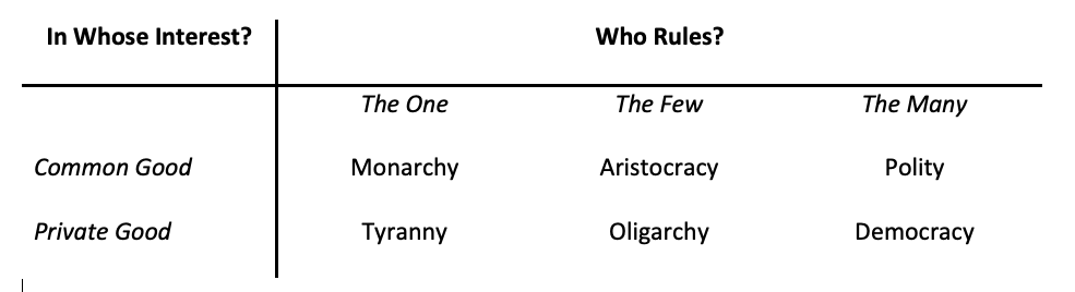
The first thing to notice is that terminology has changed since Aristotle’s time. He equated democracy with mob rule—the masses ruling in their own selfish and short-sighted interest. He also makes a different distinction than we do between aristocracy and oligarchy as though the main difference was in whose interest the few ruled. Today, we tend to see aristocracies as ruling in their selfish interest just like we do oligarchies. The main takeaway is that Aristotle thoughtfully tried to apply what he knew about political regimes in a systematic way. You can do the same thing with presidential vetoes, elections, congressional bills, political demonstrations, or just about any political phenomenon in which you have enough cases to categorize. One important rule of typologies is that the interior cells must be mutually exclusive—that is, the things that you are categorizing must fit in one—and only one—box. A political system cannot be both a polity and a monarchy in Aristotle’s typology.

References

1. Inequality.org
2. National Center for Education Statistics
3. Steve Stemler, “An Introduction to Content Analysis,” ERIC. June 2001.
4. Kenneth A. Rasinski, “The Effect of Question Wording on Public Support for Government Spending,” Public Opinion Quarterly. 53(3): Autumn, 1989. Pages 388-394.
5. Marjorie Connelly, “Push Polls, Defined,” The New York Times. June 18, 2014.